jafrog's dev blog

29 April 2024

Building A Neural Network From Scratch

Prerequisites

This walkthrough assumes that you understand the core concepts of Neural Networks. Here’s the non-exhaustive list:

Logistic regression
Gradient descent
Forward and backward propagation
Loss functions

If you understand all of the above “in principle”, but struggle to turn the concepts into code, this post is for you.

This is based on the material covered in the first course of the Deep Learning Specialisation on Coursera. I highly recommend enrolling in this course if you want to learn the fundamentals of Neural Networks. The first course in particular is a hoot.

The goal

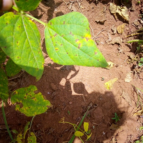
By the end of this post we should have a working Neural Network that can classify the images of beans as “heathy” or “not healthy”. The point is to understand the building blocks of a Neural Networks without using the frameworks like Tensorflow or PyTorch.

I particularly struggled with getting a good intuition for back propagation.

Next steps

In the next post we’ll change the classifier to a multi-class one using the softmax function.

The implementation

Download the dataset

# datasets is a 🤗library to load and manipulate datasets
from datasets import load_dataset

# Loads only the training examples from the dataset
dataset = load_dataset("beans", split="train")

print("Dataset shape: ", dataset.shape)
dataset[0]

Output:

Dataset shape: (1034, 3)

{
'image_file_path': '.../train/angular_leaf_spot/angular_leaf_spot_train.0.jpg',
'image': <PIL.JpegImagePlugin.JpegImageFile image mode=RGB size=500x500>,
'labels': 0
}

The shape of the dataset is (1034,3) - 1034 examples, each with 3 features: image_file_path, image and labels. The first example in the dataset has a label 0. To check what this label corresponds to, we can check the features attribute of the dataset.

dataset.features

Output:

{
'image_file_path': Value(dtype='string', id=None),
'image': Image(decode=True, id=None),
'labels': ClassLabel(names=['angular_leaf_spot', 'bean_rust', 'healthy'], id=None)
}

This dataset has 3 classes: ‘angular_leaf_spot’ = 0; ‘bean_rust’ = 1; ‘healthy’ = 2. The first example is an image of a bean leaf with angular leaf spot.

dataset[0]["image"]

Output:

Angular leaf spot

To convert the image into an input for the NN, we need to convert it into a feature vector. An RGB image is a 3D tensor with shape (height, width, channels). We can flatten this tensor into a 1D vector of shape (height * width * channels).

Convert one image to a feature vector. Each image is 500px x 500px and RGB-encoded.

from transformers import ImageFeatureExtractionMixin

feature_extractor = ImageFeatureExtractionMixin()
feature_vector = feature_extractor.to_numpy_array(dataset[0]["image"], channel_first=False)
print("Original image shape: ", feature_vector.shape)
print("Feature vector shape: ", feature_vector.flatten().shape)

Output:

Original image shape: (500, 500, 3)
Feature vector shape: (750000,)

Iterate over the dataset and convert all images to feature vectors.

We will also resize images so the feature vectors are not as long ((30000,) as opposed to (750000,))

to_numpy_array also normalizes the RGB values by default, making them between 0 and 1.

import numpy as np

def transform(examples):
    examples["feature_vector"] = [feature_extractor.to_numpy_array(image.convert("RGB").resize((100,100)), channel_first=False).flatten() for image in examples["image"]]
    return examples

dataset = dataset.map(transform, batched=True)
dataset.shape

Output:

(1034, 4)

# Convert dataset into the input for the NN
X = np.array(dataset["feature_vector"], dtype='float32').T
print("X: ", X.shape)

Output:

X: (30000, 1034)

Binary classifier

Let’s change the labels to “sick” and “not sick” to turn this into a binary classifier.

If the label is “2” the value is 0 (not sick). If it’s not “2” the value is 1 - sick.

Y = np.array([0 if label == 2 else 1 for label in dataset["labels"]])
Y.shape

Output:

(1034,)

Implementing the NN

We will define several helper functions that will implement the forward and the backward prop in the NN. These functions can account for different sizes of the network - different number of hidden layers and different number of nodes in each layer.

initialise_parameters(n_x, nn_shape) -> parameters - initialise parameters for all layers forward_prop(X, parameters) - implements the forward propagation step compute_cost(Y, Yhat) - computes cross-entropy loss back_prop - implements the back propagation step

Other helper functions: relu - RELU activation function sigmoid - sigmoid activation function relu_deriv - Computes \(\frac{\partial A}{\partial Z}\) where A is a RELU activation function sigmoid_deriv - Computes \(\frac{\partial A}{\partial Z}\) where A is a \(\sigma\) activation function

X is (30000, 1034) - model inputs. 1034 examples, each a vector of 30000 Y is (1034, 1) - outputs. Labels for each example. 0, 1 or 2.

# `nn_shape` describes the number of layers in the NN, the number of nodes in each layer and the activation function for each layer
# Note that the last layer has 1 output node since this is a binary classifier
nn_shape_binary = [
    {"nodes": 4, "activation": "relu"},
    {"nodes": 3, "activation": "relu"},
    {"nodes": 2, "activation": "relu"},
    {"nodes": 1, "activation": "sigmoid"},
]

L = len(nn_shape_binary)
m = Y.shape[0]

print("Number of layers: ", L)
print("Number of examples: ", m)

Output:

Number of layers: 4
Number of examples: 1034

def initialise_parameters(X, nn_shape):
    parameters = {}
    
    # Number of features in an example. 30000 in this case
    n_x = X.shape[0]
    
    for i, layer in enumerate(nn_shape):
        n_prev = n_x if i == 0 else nn_shape[i-1]["nodes"]
        # Use He initialisation for weights. Initially I used small random initialisation (random weights multiplied by 0.01) but it led to *significantly* worse performance.
        parameters[f"W{i+1}"] = np.random.randn(layer["nodes"], n_prev) * np.sqrt(2. / n_prev)
        # Initialise biases with zeros
        parameters[f"b{i+1}"] = np.zeros((layer["nodes"], 1))
    
    return parameters

params = initialise_parameters(X, nn_shape_binary)

for k, v in params.items():
    print(f"{k}: {v.shape}")

Output:

W1: (4, 30000)
b1: (4, 1)
W2: (3, 4)
b2: (3, 1)
W3: (2, 3)
b3: (2, 1)
W4: (1, 2)
b4: (1, 1)

def relu(Z):
    A = np.maximum(0,Z)
    
    return A

def sigmoid(Z):
    A = 1 / (1 + np.exp(-Z))
    return A

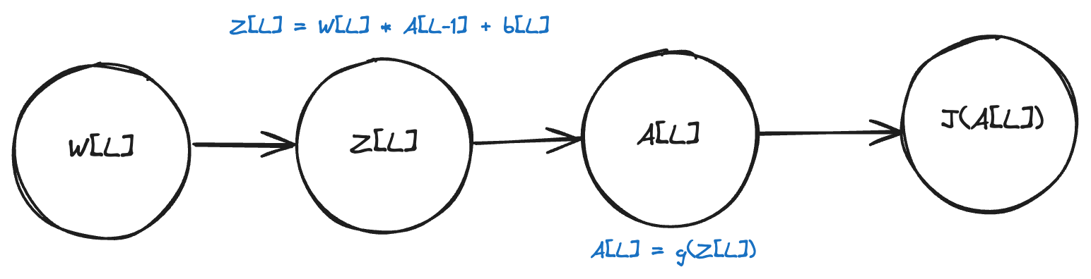
Forward propagation

In the forward propagation step, we compute two things for each layer:

Linear activation: \(Z^{[l]} = W^{[l]}A^{[l-1]} + b^{[l]}\)
Activation function: \(A^{[l]} = g^{[l]}(Z^{[l]})\)

where \(g^{[l]}\) is the activation function for layer \(l\).

activations = {
    "relu": relu,
    "sigmoid": sigmoid
}

def forward_prop(X, params, nn_shape):
    grads = {"A0": X}
    
    for l, layer in enumerate(nn_shape):
        W = params[f"W{l+1}"]
        b = params[f"b{l+1}"]
        A_prev = grads[f"A{l}"]
        
        Z = np.dot(W, A_prev) + b
        A = activations[layer["activation"]](Z)
        
        grads[f"Z{l+1}"] = Z
        grads[f"A{l+1}"] = A
        
    return grads

grads = forward_prop(X, params, nn_shape_binary)

for k, v in grads.items():
    print(f"{k}: {v.shape}")

Output:

A0: (30000, 1034)
Z1: (4, 1034)
A1: (4, 1034)
Z2: (3, 1034)
A2: (3, 1034)
Z3: (2, 1034)
A3: (2, 1034)
Z4: (1, 1034)
A4: (1, 1034)

Cost function

The cost function for a binary classifier is the cross-entropy loss:

\[J = -\frac{1}{m} \sum_{i=1}^{m} y^{(i)} \log(a^{(i)}) + (1 - y^{(i)}) \log(1 - a^{(i)})\]

where \(a^{(i)}\) is the predicted value for the \(i\)-th example and \(y^{(i)}\) is the true label for the \(i\)-th example.

The accuracy of the model can’t be derived directly from a cost function. We will compute it separately later.

# AL stands for A[L] - activation of the last layer
def compute_cost(Y, AL, m):
    # print("Compute cost shapes ", Y.shape, AL.shape)
    # Y = Y.reshape((m,))
    # AL = AL.reshape((m,))
    result = - (1/m) * (np.dot(Y, np.log(AL).T) + np.dot((1 - Y), np.log(1 - AL).T))
    return np.squeeze(result)
    
compute_cost(Y, grads[f"A{L}"], m)

Output:

0.6931471805599453

Back propagation

In the back propagation step the goal is to update the weights W and biases b in the network to minimise the cost function.

The weights and biases are updated using the gradients (partial derivatives) of the cost function with respect to the weights and biases:

\[W^{[l]} = W^{[l]} - \alpha \frac{\partial J}{\partial W^{[l]}}\] \[b^{[l]} = b^{[l]} - \alpha \frac{\partial J}{\partial b^{[l]}}\]

where \(\alpha\) is the learning rate.

Last layer with sigmoid activation function

To compute the partial derivatives of the cost function with regards to W and b, we need to apply the chain rule.

The only variable that “feeds” into the cost function is A[L]. A[L] depends on Z[L], Z[L] depends on W[L] and b[L].

Diagram 1

This means that the partial derivative of L with respect to W[L] and b[L] is computed as follows:

\[\frac{\partial J}{\partial W^{[L]}} = \frac{\partial J}{\partial A^{[L]}} \frac{\partial A^{[L]}}{\partial Z^{[L]}} \frac{\partial Z^{[L]}}{\partial W^{[L]}}\]

Let’s break down each one of these components.

dA[L]

The derivative of the cost function with respect to the activation of the last layer is computed as follows:

\[\frac{\partial J}{\partial A^{[L]}} = -\frac{Y}{A^{[L]}} + \frac{1 - Y}{1 - A^{[L]}}\]

dA[L] w.r.t Z[L]

The derivative of the activation function with respect to the linear activation of the last layer depends on the activation function g[L]. For the sigmoid activation function, it is computed as follows:

\[\frac{\partial A^{[L]}}{\partial Z^{[L]}} = \sigma'(Z^[L]) = \sigma(1 - \sigma) = A^{[L]}(1 - A^{[L]})\]

dZ[L] w.r.t W[L]

Finally, the derivative of Z[L] with respect to W[L] is the activation of the previous layer A[L-1]:

\[\frac{\partial Z^{[L]}}{\partial W^{[L]}} = A^{[L-1]}\]

Putting it all together and simpifying:

\[\frac{\partial J}{\partial W^{[L]}} = \frac{\partial J}{\partial A^{[L]}} \frac{\partial A^{[L]}}{\partial Z^{[L]}} \frac{\partial Z^{[L]}}{\partial W^{[L]}} = (-\frac{Y}{A^{[L]}} + \frac{1 - Y}{1 - A^{[L]}}) * A^{[L]}(1 - A^{[L]}) * A^{[L-1]} = (A^{[L]} - Y) * A^{[L-1]}\]

Hidden layers with RELU activation function

This is the formula I’ve struggled with the most. The derivative dZ[l] where l is one of the hidden layers. Applying the chain rule, this is how we compute dZ[l]:

Diagram 2

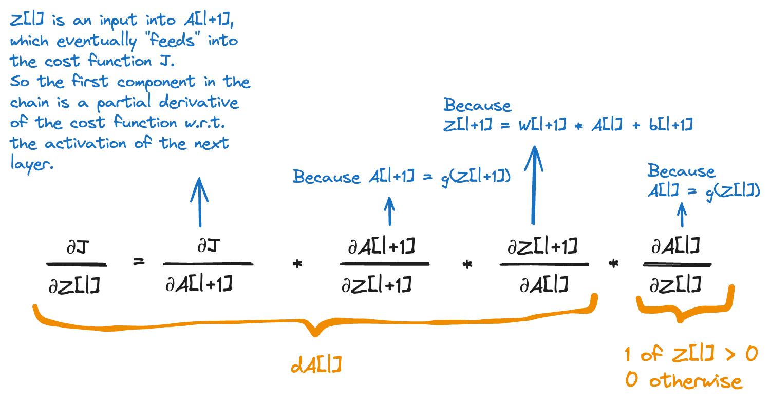
dA[l] will be multiplied item-wise with a tensor that is 1 where Z[l] is greater than 0 and 0 where Z[l] is less than or equal to 0. This is why we initialise dZ[l] to a copy of dA[l] and then set all values at the indexes where Z[l] is less than 0 to 0.

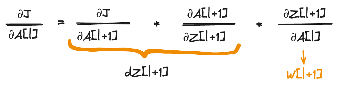
Now to compute dA[l]:

Diagram 3

def back_prop(X, Y, params, grads, nn_shape, learning_rate=0.001):
    # Number of examples
    m = Y.shape[0]
    # Number of layers
    L = len(nn_shape)
    
    # Iterate over the layers, last to first
    for l in range(L, 0, -1):
        W = params[f"W{l}"]
        b = params[f"b{l}"]
        Z = grads[f"Z{l}"]
        A = grads[f"A{l}"]

        # Compute dZ[l] for the last layer with the sigmoid activation function
        if nn_shape[l-1]["activation"] == "sigmoid":
            dZ = A - Y
        
        # Compute dZ[l] for the hidden layers
        if nn_shape[l-1]["activation"] == "relu":
            dZnext = grads[f"dZ{l+1}"]
            Wnext = params[f"W{l+1}"]
            dA = np.dot(Wnext.T, dZnext)
            grads[f"dA{l}"] = dA
            
            dZ = np.array(dA, copy=True)
            dZ[Z < 0] = 0
        
        Aprev = X if l == 1 else grads[f"A{l-1}"]
        dW = (1/m) * np.dot(dZ, Aprev.T)
        db = (1/m) * np.sum(dZ, axis=1, keepdims=True)

        W = W - learning_rate * dW
        b = b - learning_rate * db
        
        params[f"W{l}"] = W
        params[f"b{l}"] = b
        grads[f"dZ{l}"] = dZ
    
    return params

back_prop(X, Y, params, grads, nn_shape_binary)

I’m going to skip the output here, it’s a bunch of tensors.

Putting it all together

nn_shape = [
    {"nodes": 4, "activation": "relu"},
    {"nodes": 3, "activation": "relu"},
    {"nodes": 2, "activation": "relu"},
    {"nodes": 1, "activation": "sigmoid"},
]

L = len(nn_shape)
m = Y.shape[0]

num_epochs = 1000

params = initialise_parameters(X, nn_shape)

for i in range(0, num_epochs):
    grads = forward_prop(X, params, nn_shape)
    cost = compute_cost(Y, grads[f"A{L}"], m)
    params = back_prop(X, Y, params, grads, nn_shape)
    if i % 100 == 0:
        print(f"Cost at #{i}: {cost}")

Output:

Cost at #0: 0.6931471805599453
Cost at #100: 0.5647623281046791
Cost at #200: 0.49435884342270875
Cost at #300: 0.46541043351056827
Cost at #400: 0.44768665629851173
Cost at #500: 0.4339341072340277
Cost at #600: 0.4226418290681421
Cost at #700: 0.4130181578936699
Cost at #800: 0.40420962864501486
Cost at #900: 0.3960244415732821

Measuring accuracy

The accuracy of the model can not be directly derived from the cost function.

We will load the dev dataset and measure the accuracy of the model on the training and the dev set.

dev = load_dataset("beans", split="validation")
print("Dev dataset: ", dev)

dev = dev.map(transform, batched=True)

X_dev = np.array(dev["feature_vector"], dtype='float32').T
print("X_dev: ", X_dev.shape)

Y_dev = np.array([0 if label == 2 else 1 for label in dev["labels"]])

Output:

Dev dataset: Dataset({
features: ['image_file_path', 'image', 'labels'],
num_rows: 133
})
X_dev: (30000, 133)

def predict(X, params, nn_shape):
    L = len(nn_shape)

    grads = forward_prop(X, params, nn_shape)
    return grads[f"A{L}"]

def accuracy(Y, Y_pred):
    Y = np.reshape(Y, (Y.shape[0],))
    Y_pred = np.reshape(Y_pred, (Y.shape[0],))
    Y_pred_bin = (Y_pred >= 0.5).astype(int)
    return np.sum(Y == Y_pred_bin) / Y.shape[0]

Y_pred = predict(X, params, nn_shape)
Y_dev_pred = predict(X_dev, params, nn_shape)

print("Accuracy on the training set: ", accuracy(Y, Y_pred.T))
print("Accuracy on the dev set: ", accuracy(Y_dev, Y_dev_pred.T))

Output:

Accuracy on the training set: 0.8520309477756286
Accuracy on the dev set: 0.8646616541353384

That’s it! Not a bad result - ~85% accuracy on both the training and the dev set - for a small network working on a compressed images and without any optimisation.

In the next post we’ll change the classifier to a multi-class one using the softmax function.